What is the dynamic effect of monetary policy on output and prices? This is a common question asked in applied macroeconomics. Interestingly, this complex question can be addressed using relatively simple tools such as VAR, SVAR, and Local Projections. In this short article, I will walk through the basics of these three methods by setting aside the mathematical intricacies and focusing more on the intuition behind them.
VAR
Let’s begin with VAR (or reduced form VAR), which stands for Vector Autoregression. This is one of the most widely used empirical tools in macroeconomics. VAR was first introduced by Christopher Sims in the 1980s in his seminal paper, which questioned the then-dominant use of large-scale structural models. His argument was simple but powerful — in macroeconomics, most of the variables we study are endogenous, meaning they are determined together within the system, not in isolation.
The motivation behind Sims’s approach came from systems thinking. For example, if we want to study the impact of monetary policy on output, we cannot ignore the fact that monetary policy itself reacts to changes in output. So, the relationship is two-way. Traditional models treated some variables as exogenous, which often led to biased or misleading conclusions.
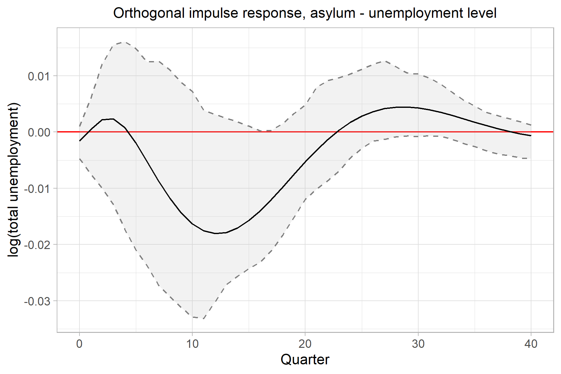
VAR handles this issue by treating all variables as potentially endogenous. It estimates a system of equations where each variable — such as consumer price index (in log scale), and real GDP (in log scale) — is regressed on its own past values as well as the past values of all other variables in the system. This allows researchers to study how a shock in one variable — say, a surprise interest rate hike — affects other variables over time. These dynamic responses are usually plotted using what are called impulse response functions.
`\pi_t` is the inflation rate
`\phi_{ij}` are the coefficients capturing dynamic interactions
`\varepsilon_{1t}` and `\varepsilon_{2t}` are the i.i.d white noise
Note: intercept terms have been suppressed for simplicity.
We can express Equation (1) and Equation (2) in the matrix form,
Here,
`F(L) = R(L)^{-1}`
Equation (3) is the VAR representation of Equation (1) and Equation (2) where `\Delta Z_t` is `2\times 1` matrix containing `y_t` and `\pi_t`. `R(L)` is the `2\times 2` matrix that captures VAR coefficients. According to the Wold Representation Theorem, any stable and invertible VAR process can be expressed in a Vector Moving Average (VMA) form by inverting the lag polynomial `R(L)`. The corresponding VMA representation can be realized by inverting `R(L)` matrix.
While VAR models describe interdependencies using lagged values of the endogenous variables, the VMA representation is often more appealing in macroeconomic applications. This is because the VMA framework isolates the role of past shocks and expresses the system in terms of serially uncorrelated reduced-form errors. This makes the dynamic propagation of shocks more transparent, even though the shocks have not yet been identified structurally. In contrast, interpreting the dynamics in a VAR model can be challenging due to the feedback loops and mutual endogeneity of the variables. $$\Delta Z_t =F(L)\mu_t---(4)$$
SVAR (Structural VAR)
SVAR is the structural extension of the traditional VAR model. It departs from the reduced-form VAR by imposing structural restrictions that are derived from economic theory or institutional knowledge. These restrictions help identify structural shocks, which are economically meaningful disturbances—such as monetary policy shocks or supply-side shocks.
The primary goal of SVAR is to map the reduced-form VAR or VMA to its structural counterpart using a contemporaneous structural matrix, typically denoted by `V`, of order `n \times n`. The order of `V` matches the order of the lag polynomial `F(L)`.
$$ \Delta Z_t = F(L) V V^{-1} \mu_t $$ $$ \Delta Z_t = B(L) \varepsilon_t \tag{5} $$
In Equation (5), `B(L) = F(L) V` captures the structural dynamics, and `\varepsilon_t` are the structural shocks. Two key features of structural shocks are:
- Orthonormality: `E[\varepsilon_t \varepsilon_t'] = I`
- Economic interpretability: Structural shocks are identified using credible economic theories or institutional assumptions.
Because the reduced-form VAR system is under-identified—meaning the number of unknowns exceeds the number of unique equations—we need additional restrictions to solve for the structural parameters. The number of restrictions required to just-identify the system is:
$$ \text{Number of restrictions} = \frac{n(n - 1)}{2} $$
Short-run Restrictions
Short-run restrictions are imposed on the contemporaneous matrix `V`. The economic rationale is that certain shocks take time to affect some variables due to rigidities, delays, or institutional frictions. These restrictions are typically zero restrictions on specific elements of `V`, meaning that a given structural shock does not have an instantaneous effect on a particular variable.
A classic example is Blanchard and Perotti (2002), who identify fiscal policy shocks using short-run restrictions. They argue that due to the time it takes to implement fiscal policy—owing to administrative and bureaucratic procedures—government spending does not respond contemporaneously to fiscal shocks. This assumption allows them to disentangle automatic responses (endogenous reactions) from exogenous fiscal policy shocks.
Long-run Restrictions
Long-run restrictions are imposed on the cumulative effects of shocks rather than their immediate (contemporaneous) effects. These are especially useful when short-run dynamics are not sufficient to distinguish among shocks.
A well-known application is Blanchard and Quah (1989), who identify demand and supply shocks in a bivariate VAR model of output and unemployment. They impose the restriction that demand shocks have no long-run effect on output. This allows them to isolate supply-side disturbances (which do have a permanent impact) from transitory demand-side fluctuations.
Mathematically, long-run restrictions are imposed on the long-run impact matrix, often derived from the infinite-horizon moving average representation of the VAR. Given that
$$ \Delta Z_t = B(L) \varepsilon_t $$
then the long-run impact matrix is:
$$ \Theta = \sum_{j=0}^{\infty} B_j $$
Local Projections
To be continued...


Post a Comment