
In applied econometrics, researchers often encounter situations where conventional standard errors may produce biased inference. This can happen, for instance, when error terms are not normally distributed, when the sample size is small, or when the analytical expression of the standard error is unknown. In such cases, relying on conventional methods is inappropriate, and alternative approaches—such as bootstrap techniques—are required to obtain valid inference. In this post, I start with the intuition behind the bootstrap and then provide a concise overview of its various types along with practical example in Python.
Concept of Bootstrap
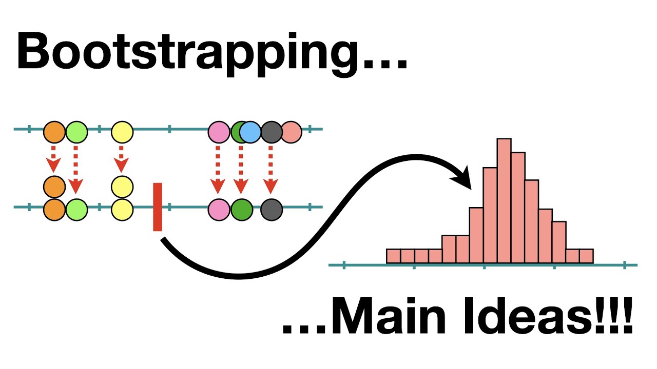
The bootstrap is a method that helps us understand how uncertain a statistic is, using only the data we have. Instead of relying on complicated formulas or strict assumptions, it works by repeatedly resampling our data with replacement to create many “new” datasets, calculating the statistic each time. The spread of these results tells us how much the number could vary, giving us a practical way to measure confidence or error.
Let us illustrate the bootstrap with a simple example. Suppose we have a dataset containing the ages of 1,000 individuals from an unknown population. One way to estimate the true population mean is by using the bootstrap.
Here’s how it works:
- Resample the data with replacement `n` times (for example, 1,000 bootstrap samples).
- For each resampled dataset, we calculate the mean age.
- Collect all these means and calculate their average—this gives the bootstrap estimate of the population mean.
- The standard deviation of these bootstrap means provides the bootstrap standard error, which measures the uncertainty of our estimate.
This approach allows us to approximate the sampling distribution of the mean without making strong assumptions about the underlying population.
Now, I implement the bootstrap in Python with hypothetical data.
This video provides an intuitive explanation of bootstrapping.
Bootstrap methods
Now, I will walk through various bootstrap methods and how to implement them in regression framework.
1. Simple or Classic Bootstrap
Suppose we have a dataset with two variables, `y` and `x`, containing 25 observations. We estimate the regression equation:
$$y = \alpha + \beta x + \epsilon$$
Our goal is to estimate the standard error of `\beta` using both simple OLS and the bootstrap.
We perform `B = 1000` bootstrap replications as follows:
- First, randomly resample 25 observations (`y_i, x_i`) with replacement from the original dataset.
- Second, estimate the regression coefficient `\hat{\beta}^{(b)}` from the resampled data.
- Third, store `\hat{\beta}^{(b)}`.
After completing all bootstrap replications, we calculate:
The bootstrap mean of the coefficients:
$$\bar{\beta} = \frac{1}{B} \sum_{b=1}^B \hat{\beta}^{(b)}$$
The bootstrap standard error as the standard deviation of the stored coefficients:
$$SE_{\text{boot}}(\hat{\beta}) = \sqrt{\frac{1}{B-1} \sum_{b=1}^B \left( \hat{\beta}^{(b)} - \bar{\beta} \right)^2}$$
Here, `SE_{\text{boot}}(\hat{\beta})` is the bootstrap estimate of the standard error of `\beta`.
Now, let us implement this procedure in python.
Though this procedure is straightforward, it is highly prone to failure when the predictor is a highly imbalanced binary variable. Using the sample dataset, I demonstrate how bootstrap failures occur in such cases.
Why does the bootstrap fail in this example? To answer this, recall the OLS formula for `\hat{\beta}`:
$$\hat{\beta} = \frac{\text{cov}(y, x)}{\text{var}(x)}$$
The bootstrap fails here because `x` is a highly imbalanced binary variable: 23 observations have `1` and only 2 observations have `0`. Bootstrap resamples the data randomly with replacement, so it is likely that some resampled datasets will contain only `1`s. In that case, both covariance of `y` and `x` and variance of `x` becomes zero, making `\hat{\beta}` indeterminate. In our example, 119 out of 1000 bootstrap replications failed, which means that 119 times out of 1000 the resampled `x` contained only `1`s.
2. Residual Bootstrap
Bootstrap failure is a common issue when working with highly imbalanced binary regressors. In such cases, the standard bootstrap can produce samples in which the predictor `x` has no variation, making the coefficient estimate `β̂` indeterminate. One effective way to overcome this problem is to use the residual bootstrap, which keeps `x` fixed and only resamples the residuals. The procedure can be described step by step as follows:
- Run the original OLS: We estimate the regression `y = α + β x + ε` using the original data and obtain the fitted values `ŷ` and the residuals `ε̂ = y - ŷ`. These residuals capture the variation in `y` that is not explained by `x`.
- Resample residuals: We randomly sample (with replacement) from the residuals `ε̂` to create a new set of residuals `ε̂^*`. Then, we add these resampled residuals to the original fitted values to construct a new dependent variable:
$$y^* = \hat{y} + \hat{\epsilon}^*$$
This ensures that the new `y^*` maintains the same relationship with `x` as the original data while introducing variability through the resampled residuals.
- Run OLS on the new dataset: We regress `y^*` on the original `x` and obtain the coefficient estimate `β̂^*`. Because `x` is kept fixed, there is always variation in the predictor, preventing the bootstrap failure encountered with highly imbalanced binary regressors.
- Repeat the procedure: We repeat steps 2–3 for `B` bootstrap replications and collect all the `β̂^*` estimates to form the bootstrap distribution of `β̂`. From this distribution, we can compute standard errors, confidence intervals, and other inferential statistics.
By keeping the predictor `x` fixed and resampling only the residuals, the residual bootstrap avoids the problem of zero variance in `x` and provides more reliable inference when working with highly imbalanced binary variables.
3. Wild bootstrap
- Run the original OLS: We estimate the regression `y = \alpha + \beta x + ε` using the original data and obtain the fitted values `ŷ` and the residuals `ε̂ = y - ŷ`. These residuals capture the variation in `y` that is not explained by `x`.
- Draw Rademacher weights: For each observation
i = 1, 2, ..., n, draw a random variablewᵢthat takes the values +1 or −1 with equal probability:
- Create Bootstrap Errors: Form the bootstrap error for each observation: $$ \varepsilon_i^{*} = w_i \times \hat{\varepsilon}_i $$This equation multiplies each residual `\hat{\varepsilon}_i` by its randomly drawn weight `w_i` (either +1 or −1). By doing so, the magnitude of each residual—and thus any heteroskedastic pattern in the data—remains intact, while the sign is randomized. This is what allows the wild bootstrap to properly handle heteroskedasticity.
- Generate new y: Constructing the new dependent variable: $$y_i^{*} = \hat{y}+ \varepsilon_i^{*}$$
- Refit the model: Now, we re-estimate the model with new dependent variable$$y_i^{*}=\gamma + \theta x_i + \nu_i$$Store `\hat{\theta}`.
- Repeat: Repeat above steps `B` times, generally 1000 times and store `\hat{\theta}`. Therefore, we have `B` `\hat{\theta}`.$$\hat{\theta_1},\hat{\theta_2},...,\hat{\theta_B}$$ Finally, compute bootstrap mean and standard error as usual.
4. Wild cluster bootstrap
- Run the original OLS: We estimate the regression `y_{ig} = \alpha + \beta x_{ig} + \varepsilon_{ig}` using the original data and obtain the fitted values `ŷ_{ig}` and the residuals `\hat{\varepsilon_{ig}}= y_{ig} - ŷ_{ig}`. These residuals capture the variation in `y` that is not explained by `x`. Here, `i` denotes individual units and `g` denotes groups or clusters.
- Draw Rademacher weights: For each observation
i = 1, 2, ..., n, draw a random variable `w_g` that takes the values +1 or −1 with equal probability at cluster level:
- Create Bootstrap Errors: Form the bootstrap error for each observation: $$ \varepsilon_{ig}^{*} = w_g \times \hat{\varepsilon}_{ig} $$This equation multiplies each residual `\hat{\varepsilon}_{ig}` by its randomly drawn weight at cluster level, `w_g` (either +1 or −1). By doing so, the magnitude of each residual within each cluster—and thus any heteroskedastic pattern as well as common shocks in the data—remains intact, while the sign is randomized. This is what allows the wild cluster bootstrap to properly handle heteroskedasticity under cluster specific common shocks.
- Generate new y: Constructing the new dependent variable: $$y_i^{*} = \hat{y}+ \varepsilon_{ig}^{*}$$
- Refit the model: Now, we re-estimate the model with new dependent variable$$y_{ig}^{*}=\gamma + \theta x_{ig} + \nu_{ig}$$Store `\hat{\theta}`.
- Repeat: Repeat above steps `B` times, generally 1000 times and store `\hat{\theta}`. Therefore, we have `B` `\hat{\theta}`.$$\hat{\theta_1},\hat{\theta_2},...,\hat{\theta_B}$$ Finally, compute bootstrap mean and standard error as usual.
Post a Comment